Geometry definition

A Geant4 Monte Carlo geometry consists of a hierarchy of nested G4VPhysicalVolumes, starting from a single root (“World”) volume. Calzone represents this structure using base Python objects (bool, dict, float, int, list and str) that have associated representations in common configuration languages, such as JSON, TOML or YAML.

In the following section, we illustrate Calzone’s geometry representation with some of the examples distributed with the source. For a more comprehensive account of the Calzone geometry definition, please refer to the Reference section hereafter.

Note

While Calzone supports various geometry formats, the examples provided in this section are all in TOML format.

---

Examples

Flat air-soil interface

To begin with a basic example, let us consider a flat air-soil interface (as in the gamma/benchmark example). This is represented with Calzone using a geometry.toml file, with the following content

[Environment]
box = 2E+05
material = "G4_AIR"

[Environment.Ground]
box = [2E+05, 2E+05, 1E+05]
position = [0.0, 0.0, -5E+04]
material = "G4_CALCIUM_CARBONATE"

The root volume is defined by an axis-aligned cubic box of 2 km extension (i.e. 2E+05 cm), named Environment and filled with "G4_AIR" (from the Geant4 NIST database). The root volume (Environment) contains a daughter volume (Ground), which is also of box shape, with a square base of 2 km sides and a height of 1 km. The origin (i.e. the box centre) of the Ground volume is offset by 500 m along the z-axis w.r.t. its mother volume (as specified by the position attribute). As a result, the Ground volume occupies the lower half of the root volume.

Tip

Calzone supports various volume shapes, not only boxes. Please refer to the Shape definition section below for a description of the available volume shapes.

Following the same box logic, a second Detector volume (\(20 \times 20 \times 10 \, \mathrm{m}^3\)) is placed within the root volume, with its base positioned 5 cm above the top of the ground volume. This is achieved as

[Environment.Detector]
box = [2E+03, 2E+03, 1E+03]
position = [0.0, 0.0, 5.05E+02]
material = "G4_SODIUM_IODIDE"

The resulting geometry is represented in Fig. 1 below.

Warning

It is the user’s responsibility to ensure that daughter volumes do not collide with each other or with their mother volume. This can be tested by running the Geometry.check method.

(A)

(B)

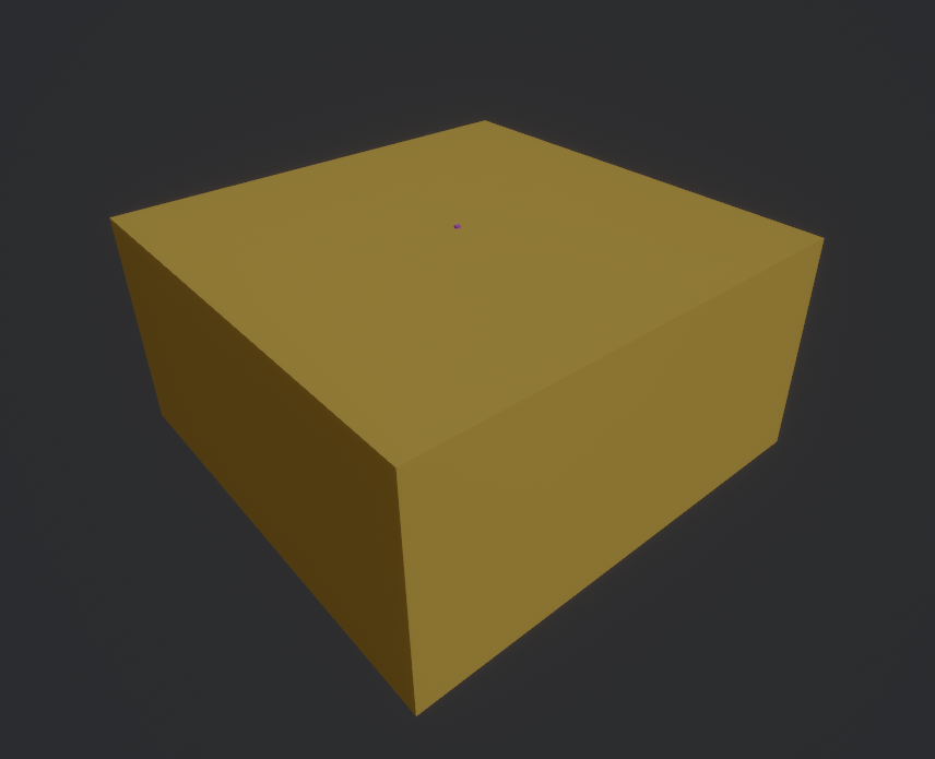
Fig. 1 Representations of the gamma/benchmark example. (A) Cross-section along the (xOz) plane. (B) Calzone display view (the root volume is transparent).

Including a topography

Let us now consider a more realistic example, in which the air-soil interface is described by a Digital Elevation Model (DEM), as in the geometry/topography example. The corresponding TOML geometry file is

[Environment]
envelope = { shape = "box", padding = [ 0, 0, 0, 0, 0, 3e4 ] }

[Environment.Terrain]
mesh = { path = "meshes/terrain.png", units = "m", padding = 200 }
material = "SomeRock"

[materials.mixtures]
SomeRock = { density = 2.0, state = "solid", composition = { StandardRock = 1 }}

This example introduces two new shapes that are specific to Calzone. Firstly, the root volume is defined as a box-like Envelope Shape. This is a dynamic shape whose extent adapts to its content. The padding attribute indicates that the envelope should reserve 300 m of additional space along the upward direction (i.e., along the z-axis), for the atmosphere above the ground.

Secondly, the ground is represented by the Terrain volume using a Mesh Shape. The corresponding mesh is built from the DEM specified in "meshes/terrain.png", whose system of units is metres. The DEM describes a surface, \(z = f(x, y)\), which needs to be closed in order to be a valid Geant4 volume. This is achieved by completing the DEM surface with five axis-aligned flat faces in order to form a box-like base. In this situation, the padding attribute specifies that the bottom face should be located 200 map units (i.e. metres) below the minimum height of the DEM surface. The resulting geometry is represented in Fig. 2 below.

In addition, the Terrain uses a custom "SomeRock" material whose definition is inlined below. It is a derivative of the PDG standard rock, with a lower density, e.g. representing a porous rock.

(A)

(B)

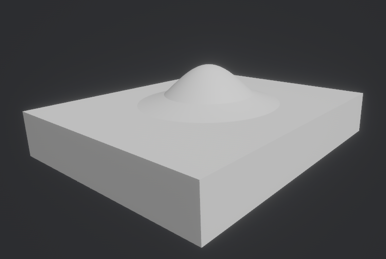
Fig. 2 Representations of the geometry/topography example. (A) Cross-section along the (xOz) plane. (B) Calzone display view (the root volume is transparent).

Replicating a volume

Finally, let us consider the case of replicating a composite volume at different locations, as with the muon/trajectograph example. In this use case, we consider a toy muography detector made of four identical detection planes (i.e. replicas) and a central lead-scatterer (to reject low-energy background particles). Replication is achieved by delegating the description of a single detection plane to an auxiliary file (layer.toml), which is included four times in the main geometry file, as below

[Detector]
include = [
    { name = "Layer0", path = "layer.toml", position = [ 0.0, -90.0, 0.0 ], rotation = [ 90.0, 0.0, 0.0 ] },
    { name = "Layer1", path = "layer.toml", position = [ 0.0, -30.0, 0.0 ], rotation = [ 90.0, 0.0, 0.0 ] },
    { name = "Layer2", path = "layer.toml", position = [ 0.0,  30.0, 0.0 ], rotation = [ 90.0, 0.0, 0.0 ] },
    { name = "Layer3", path = "layer.toml", position = [ 0.0,  90.0, 0.0 ], rotation = [ 90.0, 0.0, 0.0 ] },
]

[Detector.Scatterer]
material = "G4_Pb"
box = [ 120.0, 10.0, 130.0 ]

Note that an included geometry may itself include sub-geometries. For instance, in the current example, a detection plane is composed of six identical sub-units (named muon chambers), as below

[Layer]
material = "G4_AIR"
envelope = "box"

include = [
    { name = "Chamber00", path = "chamber.toml", position = [ -26.325, -36.0, 0.0 ] },
    { name = "Chamber01", path = "chamber.toml", position = [ -26.325,   0.0, 0.0 ] },
    { name = "Chamber02", path = "chamber.toml", position = [ -26.325,  36.0, 0.0 ] },
    { name = "Chamber10", path = "chamber.toml", position = [  26.325, -36.0, 0.0 ], rotation = [ 0.0, 0.0, 180.0 ] },
    { name = "Chamber11", path = "chamber.toml", position = [  26.325,   0.0, 0.0 ], rotation = [ 0.0, 0.0, 180.0 ] },
    { name = "Chamber12", path = "chamber.toml", position = [  26.325,  36.0, 0.0 ], rotation = [ 0.0, 0.0, 180.0 ] },
]

where the chamber.toml file contains the geometry description of a muon chamber. The resulting geometry is represented in Fig. 3 below.

(A)

(B)

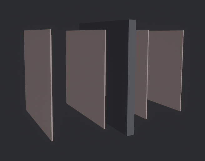
Fig. 3 Representations of the muon/trajectograph example. (A) Cross-section along the (yOz) plane. (B) Calzone display view (the root volume is transparent).

---

Reference

Geometry objects

All geometry objects (volumes, shapes, materials, etc.) adhere to the same data structure. A geometry object is represented by a Python dict item (i.e. a [key: str, value: dict] pair), where the key is the object name, and the value might be another dict, e.g. containing the object’s properties. To illustrate, a 1 cm³ cubic box shape writes,

box = { size = [ 1.0, 1.0, 1.0 ] }

Objects names

The objects proper names (i.e. designating specific volumes, materials, etc.) must be capitalised and comprise solely alpha-numeric characters. Thus, names are typically upper CamelCased. Conversely, common names (designating properties, shape types, etc.) adhere to the snake_case syntax.

Substitution rules

For the sake of convenience, the values of geometry objects are subject to certain substitution rules, which are listed in Table 2. To illustrate, a path-str (refering to a file) can be substituted for any dict value. Another useful rule is that a size-one dict whose item key can be inferred, can be substituted with the item value. This occurs, for instance, for object values that have a single mandatory property. Thus, using substitution rules, the previous cubic box shape simplifies as,

box = 1.0

Table 2 Substitution rules.

Type	Substitute	Comment
dict	str	"*.json", "*.toml" or "*.yaml".
{ key: value }	value	If the key can be inferred.
[T; N]	T	E.g., 1.0 -> [ 1.0, 1.0, 1.0 ].
[T]	T	E.g., "Detector" -> [ "Detector" ].
[[float; 3]; 3]	[float; 3]	Rotation vector (with angles in deg).

Relative path

As a particular case of substitution rule, path-str, pertaining to included files, are relative to the directory in which the including file is located, unless an absolute path is specified.

Geometry structure

A geometry definition starts with a root volume, for instance as follows,

[RootName]

box = 1.0
..

There can be only one root volume in a geometry. However, the geometry dict might contain the additional "materials" and "meshes" keys, for describing the geometry materials and specific triangle meshes. The corresponding structure is summarised below, in Table 3.

Table 3 Geometry items.

Key	Value type	Default value
RootName	dict (Table 4)
"materials"	dict (Table 15)	None
"meshes"	dict (Table 14)	None

Pathname

Geometry volumes are identified by their absolute pathname, which is formed by the dot-jointure of their own name with all of their ancestors names. For example, the "Environment.Detector" pathname refers to the "Detector" volume located inside the "Environment" volume.

The dict representation of the geometry ensures that pathnames are unique within a given geometry.

Volume definition

The items of a Monte Carlo volume are presented in Table 4 below. If no shape is specified, then a box envelope is assumed. To illustrate, a 1 cm³ cubic box volume filled with water would be represented as follows,

[VolumeName]

material = "G4_WATER"
box = 1.0

Note that a volume can only have a single shape item (but multiple daughter volumes). For further information on shape types and their corresponding items, see Shape definition.

Table 4 Volume items.

Key	Value type	Default value
"material"	str	"G4_AIR"
shape_type	dict (Shape items)	"envelope"
"position"	[float; 3]	numpy.zeros(3)
"rotation"	[[float; 3]; 3]	numpy.eye(3)
"role"	[str]	None
"disentangle"	dict (Table 6)	None
"subtract"	[str]	None
DaughterName	dict (Table 4)	None
"include"	[dict] (Table 7)	None
"materials"	dict (Table 15)	None
"meshes"	dict (Table 14)	None

Positioning properties.

The optional "position" and "rotation" properties are relative to the mother volume frame. By default, the volume is placed unrotated with its origin coinciding with the mother one.

Daughter volumes.

The daughter volumes are included directly with the volume properties. They are identified by their CamelCase syntax.

Materials and meshes definitions.

Materials and meshes can be defined together with the volume properties, should this be required. It should be noted, however, that they exist on a global level, regardless of their definition scope (see the Materials and Meshes definition sections for further information).

Roles

By default, geometry volumes are inert, i.e. they do not record any Monte Carlo information. The "role" property can be used to assign specific tasks. A volume role is formed by a two words snake-cased sentence starting with a verb (the action), and followed by a subject (the recipient). For example, the following indicates that the volume should record energy deposits, and capture outgoing particles.

role = [ "record_deposits", "catch_outgoing" ]

Possible actions and recipients are listed in Table 5 below.

Table 5 Volume roles vocabulary.

Word	Nature	Description
"catch"	Verb	Extract Monte Carlo particles at the volume boundary.
"kill"	Verb	Silenty kill Monte Carlo particles at the volume boundary.
"record"	Verb	Record energy deposits and/or Monte Carlo particles.
"all"	Subject	Designates both energy deposits and particles.
"deposits"	Subject	Designates only energy deposits.
"ingoing"	Subject	Designates only ingoing particles.
"outgoing"	Subject	Designates only outgoing particles.
"particles"	Subject	Designates both ingoing and outgoing particles.

Note

Unlike other geometric properties, roles are not fixed. E.g., they can be modified after the Monte Carlo geometry has been loaded (see the Volume.role attribute).

Overlaps

The "disentangle" and "subtract" volume properties address the issue of overlaps between sister volumes in two distinct ways. The "subtract" property explicitly specifies sister volumes (by their name) whose shape are to be subtracted from the current volume. This can be employed, for instance, to dig out a portion of a "Ground" volume to accommodate a partially buried "Detector" volume.

Note

Only unsubtracted volumes can be subtracted from. Consequently, the subtract property does not permit the formation of subtraction chains.

The "disentangle" property indicates pairs of overlapping daughter volumes which should be separated, (see Table 6), for instance as,

[VolumeName.disentangle]

Bottom = [ "Left", "Right" ]
Top = "Left"

These volumes are separated using an iterative subtraction procedure. It should be noted that this procedure does not guarantee which volume is subtracted or not. It is therefore recommended that this method be used only for the purpose of patching small (erroneous) overlaps (e.g. due to numeric approximations).

Table 6 Disentangle items.

Key	Value type	Default value
VolumeName	[str]

Includes

The "include" volume property permits the insertion of sub-geometries, defined in auxiliary files, as daughter volumes. For example, as

[MotherName]

include = "relative/path/to/a/daughter/geometry.toml"

Some of the properties of the included root volume can be overridden, as detailed in Table 7 below. The following example explicitly sets the name of the included root volume.

[MotherName]

include = { name = "DaughterName", path = "relative/path/to/a/daughter/geometry.toml" }

Table 7 Include items.

Key	Value type	Default value
"path"	str
"name"	str	None
"position"	[float; 3]	numpy.zeros(3)
"rotation"	[[float; 3]; 3]	numpy.eye(3)
"subtract"	[str]	None

Shape definition

The available shape types are described below. Calzone only exports a limited number of the G4VSolids defined by Geant4, namely the box, cylinder and sphere shapes. For more complex use cases, meshes should be employed.

Note

Shape type names follow the snake_case syntax (i.e. like property names).

Box shape

An axis-aligned box (G4Box), centred on the origin, and defined by its size (in cm) along the x, y and z-axis.

Table 8 Box items.

Key	Value type	Default value
"size"	[float; 3]

Cylinder shape

A cylinder of revolution around the z-axis (G4Tubs), centred on the origin, and defined by its length (in cm) along the z-axis and its radius (in cm) in the xOy plane.

Table 9 Cylinder items.

Key	Value type	Default value
"length"	float (cm)
"radius"	float (cm)
"thickness"	float (cm)	None
"section"	[float; 2] (deg)	None

Hollow cylinder.

If thickness is not None, then the cylinder is hollow (i.e. actually a tube, with the specified thickness).

Cylindrical section.

The optional section argument specifies the angular span of the cylindrical shape (in deg). By default, the cylinder is closed, i.e. it spans the whole azimuth angle ([0, 360] deg).

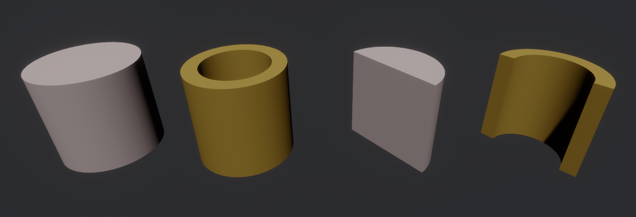
Fig. 4 Examples of cylindrical shapes visualised with Calzone display. The gold shapes are hollow cylinders, while the silver ones are plain cylinders. The shapes on the right are cylindrical sections, while those on the left are full cylinders.

Envelope shape

A bounding envelope with a specified shape, whose size is determined by the bounded daughter volumes. The padding parameter (in cm) allows for extra space around bounded objects.

Table 10 Envelope items.

Key	Value type	Default value
"padding"	[float; 6]	0.01 (cm)
"shape"	str	"box"

Padding

The padding parameter specifies additional space along the \(-X\), \(X\), \(-Y\), \(Y\), \(-Z\), and \(Z\) axes, in that order. As a special case, the padding can also be specified as a length-3 array with elements corresponding to the \(\pm X\), \(\pm Y\), and \(\pm Z\) axes. A single float parameter can also be specified, following the usual substitution rules, resulting in uniform padding along the 6 directions.

Mesh shape

A triangle mesh defined from a data file (path property) with the specified length units.

Table 11 Mesh items.

Key	Value type	Default value
"path"	str
"algorithm"	str	None
"units"	str	"cm"

The actual shape depends on the data file format. If the file is a native 3D model (in OBJ or STL format), then the mesh is directly imported. Alternatively, the data can also be a surface described by a Digital Elevation Model (DEM), in GeoTIFF or Turtle / PNG [NBCM20] format. In this case, elevation values are assumed to be along the z-axis, and the surface is closed by adding side and bottom faces. The additional properties described in Table 12 control the generated 3D shape.

Algorithm

The algorithm property specifies the method used to traverse the mesh. The available options are "bvh" or "voxels" (Geant4 method). The BVH method is an efficient solution for penetrating particles (photons, muons, etc.). However, if short-range secondaries are also simulated (e.g. electrons), the Voxels method is a more efficient CPU-wise solution, though it requires more memory (which prevents using this method with large meshes).

If no algorithm is specified, "voxels" is used for native 3D meshes and "bvh" for DEMs. See also the algorithm attribute of the GeometryBuilder class, which allows for the global override of the mesh traversal algorithm across the entire geometry.

Table 12 DEM specific items.

Key	Value type	Default value
"padding"	float	100.0 (in map units)
"origin"	[float; 3]	numpy.zeros(3)
"regular"	bool	False

Geometric properties.

The origin property defines the origin of the 3D shape in the DEM coordinates system. The padding property extends the shape below the DEM’s minimum elevation value.

Meshing type.

The regular flag controls the meshing algorithm. By default, a non-regular -but optimised- mesh is used. However, this is not supported by the Geant4 traversal algorithm. Therefore, a regular mesh must be selected when using the latter algorithm.

Tip

The Map.dump() method allows one to export the generated 3D topography in STL format.

Sphere shape

A sphere (G4Orb or G4Sphere), centred on the origin, and defined by its radius (in cm).

Table 13 Sphere items.

Key	Value type	Default value
"radius"	float
"thickness"	float (cm)	None
"azimuth_section"	[float; 2] (deg)	None
"zenith_section"	[float; 2] (deg)	None

Hollow sphere.

If thickness is not None, then the sphere is hollow, with the specified thickness value.

Spherical section.

The optional azimuth_section and zenith_section arguments specify the angular span of the spherical shape (in deg). By default, the sphere is closed, i.e. it spans the whole azimuth angle ([0, 360] deg), and the whole zenith angle ([0, 180] deg).

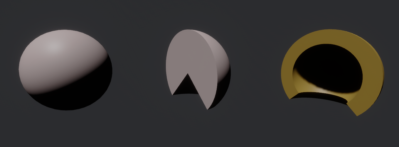
Fig. 5 Examples of spherical shapes visualised with Calzone display. The gold shape is a hollow sphere, while the silver ones are plain spheres. The shape on the left is a full sphere, while those on the left are spherical sections.

Meshes definition

Mesh shapes can be explicitly assigned a name, enabling cross-referencing. This is achieved by first defining a mesh name along with its attributes under the meshes field (in accordance with Table 14 below). Subsequently, the designated mesh name can be utilized as a shape value in volume definitions, in lieu of a dictionary description. For instance,

[meshes]
Screw = { path = "/path/to/screw.stl", units = "mm" }

[LeftScrew]
material = "Steel"
mesh = "Screw"
position = [ -3.0, 0.0, 0.0]

[RightScrew]
material = "Steel"
mesh = "Screw"
position = [  3.0, 0.0, 0.0]

Table 14 Meshes items.

Key	Value type	Default value
MeshName	dict (Table 11)	None

Meshes scope

Meshes are shared across all geometries, even when anonymous. Calzone takes care of sharing mesh data, instead of duplicating them.

Materials definition

A Geant4 material (G4Material) can be defined either as an assembly of atomic elements (G4Elements), denoted Molecule herein, or as a Mixture of other materials.

Tip

A collection of standard atomic elements and materials is readily available from the Geant4 NIST database. For example, "G4_WATER", "G4_AIR", etc. In addition, Calzone also predefines "StandardRock" (following the PDG ). Thus, depending on your application, you may not need to define your own materials.

Tip

In addition to the JSON, TOML and YAML formats, Calzone also supports importing materials from a Gate DB file.

Materials scope

Geant4 materials are defined on a global scale and are applicable to all geometries and physics. Each material is identified by a unique name. Once instanciated by Geant4, a material cannot be deleted or modified.

Materials table

The structure of a materials table is described by Table 15 (et al.) below. Molecules and Mixtures are explictily separated. For instance,

[molecules]

H2O = { .. }

[mixtures.Air]

density = 1.205E-03
..

In addition, the materials table may also contain (custom) atomic elements.

Table 15 Materials items.

Key	Value type	Default value
"elements"	dict (Table 16)	None
"molecules"	dict (Table 17)	None
"mixtures"	dict (Table 18)	None

Table 16 Atomic elements items.

Key	Value type	Default value
ElementName	dict (Table 19)

Table 17 Molecules items.

Key	Value type	Default value
MoleculeName	dict (Table 20)

Table 18 Mixtures items.

Key	Value type	Default value
MixtureName	dict (Table 22)

Atomic elements

Atomic elements are specified by their atomic number (Z) and by their mass number (A, in g/mol). Optionally, a symbol can be specified.

Table 19 Atomic element items.

Key	Value type	Default value
"Z"	float
"A"	float
"symbol"	str	None

Molecules

Molecules are defined by their density (expressed in in g/cm³) and their atomic elements composition. Additionally, a state may be specified ("gas", "liquid" or "solid"). In the absence of an explicit composition specification, it is inferred from the molecule name, which is interpreted as a chemical formula. For example,

[molecules]

H2O = { density = 1.0, state = "liquid" }

Table 20 Molecule items.

Key	Value type	Default value
"density"	float
"composition"	dict (Table 21)	None
"state"	str	None

Table 21 Molecule component.

Key	Value type	Default value
ElementName	int

Mixtures

Mixtures are specified by their density (in g/cm³) and their mass composition. Optionaly, a state can be specified ( "gas", "liquid" or "solid"). For instance,

[mixtures.Air]

density = 1.205E-03
state = "gas"
composition = { N = 0.76, O = 0.23, Ar = 0.01 }

Table 22 Mixture items.

Key	Value type	Default value
"density"	float
"composition"	dict (Table 23)
"state"	str	None

Table 23 Mixture component.

Key	Value type	Default value
ElementName	float
MaterialName	float